Recurrent Structural Policy Gradient for Partially Observable Mean Field Games

Clarisse Wibault

May 2026

Paper | Code | Google Colab

In this post, I will introduce Recurrent Structural Policy Gradient (RSPG), a Hybrid Structural Method that learns history-dependent policies for Partially Observable Mean Field Games with Public Information.

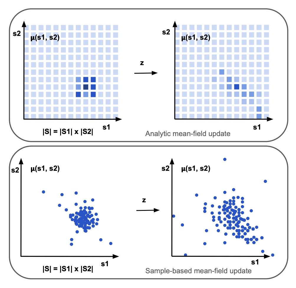
Analytic vs. Sample Based Mean Field Update

Figure 2: Top: Analytic mean-field update. Bottom: Sample-based mean-field update.

Many real-world systems involve large populations of interacting agents, such as investors responding to stock prices, households reacting to interest rates, or individuals adapting to reported infection levels during an epidemic. Mean-Field Games (MFGs) provide a principled framework for modelling these interactions. By assuming that individuals respond only to the aggregate behaviour of other agents, MFGs reduce the analysis of a large population model to the interaction between a stand-in agent and the mean field $\mu_t$.

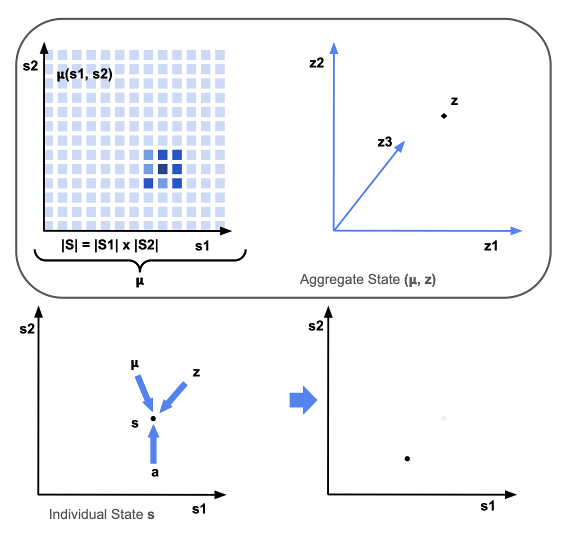
Figure 1: Top Left: the mean-field is a distribution over a (low-dimensional) individual state space. Top Right: the common noise $z_t$ is the same for all agents and can be arbitrarily high-dimensional. Bottom Left: an agent in a certain state $s_t$ takes an action $a_t$, and transitions to a new state $s_{t+1}$ conditioned on the aggregate state $(\mu_t, z_t)$.

In MFGs with common noise, uncertainty enters through aggregate shocks that affect the entire population simultaneously. While idiosyncratic noise marginalises out at the population level, common noise induces stochastic evolution of the mean-field. The resulting Markovian aggregate state $(\mu_t, z_t)$ consists of the mean-field $\mu_t$, a distribution over the individual state space $\mathcal{S}$, and the common noise $z_t$, which captures all remaining state components.

The analytic mean-field update conditions on a particular realisation of the common noise:

Analytic Mean-Field Update (Fully Observable)

$$\mu_{t+1}(s_{t+1}) = \int_{\mathcal{S}} \int_{\mathcal{A}} \mathcal{T}(s_{t+1}\mid s_t, a_t, \mu_t, z_t)\pi(a_t \mid s_t, \mu_t, z_t)\mu_t(s_t)\mathrm{d}a_t\mathrm{d}s_t$$

Or, in vector-matrix form:

$$\boldsymbol{\mu}_{t+1} = {\mathbf{A}^\pi_{\mu_t, z_t}}^\top\boldsymbol{\mu}_t.$$

In partially observable MFGs, agents must infer the aggregate state $(\mu_t, z_t)$ rather than observing it directly. As summarised by the following assumption, in many applications of interest, agents only receive a shared partial observation of the aggregate state. For example, the public information might be stock prices, interest rates, reported infection levels or communication signals.

Assumption 1: Structural Assumption - Public Partial Information

Agents receive a shared partial observation of the aggregate state: $o_t = \mathcal{U}(\mu_t, z_t)$.

The issue is that existing methods for modelling large population systems typically address only subsets of these three challenges posed by mean-field interaction, common noise, and partial observability. Deep Reinforcement Learning (RL) approaches for MFGs with common noise could trivially incorporate memory through recurrence to handle partial observability, but, as demonstrated in the following section, these methods are model-free and therefore do not exploit known system structure for variance reduction.

Dynamic Programming, Reinforcement Learning & Hybrid Structural Methods

In MFGs with common noise, the policy is usually updated by computing the value associated with the current policy and then taking a greedy step to improve that policy.

We now briefly describe policy evaluation using Dynamic Programming (DP), Reinforcement Learning (RL) and Hybrid Structural Methods (HSMs), which respectively leverage full, no or partial knowledge of the model.

Dynamic Programming (DP)

Ideally, since transition dynamics are known by modelling assumption, we would use DP to compute the value. DP leverages full access to the model i.e. both the individual state dynamics $\mathcal{T}(s'\mid s, a, \mu, z)$ and common noise dynamics $\Xi(z'\mid z)$.
White-box access to individual-state transition dynamics means that the induced mean-field sequence is computed analytically:

$$ {\boldsymbol{\mu}' = {\mathbf{A}}^{\pi}_{\mu, z}}^\top \boldsymbol{\mu}.$$

It evaluates exact expected returns through the infinite-dimensional Bellman equation or Master Equation:

$$ V(s,\boldsymbol{\mu},z) = \mathbb{E}_{a \sim \pi} \left[ R(s,a, \boldsymbol{\mu},z) + \gamma \mathbb{E}_{s' \sim \mathcal{T}, z' \sim \Xi} \left[V(s',\boldsymbol{\mu}', z')\right]\right]. $$

By evaluating the policy using exact expected returns, the Master Equation eliminates sample variance. But, in practice, integrating over all possible realisations of the mean-field due to different realisations of the common noise renders DP intractable.

Reinforcement Learning (RL)

RL treats transitions as a black-box and relies purely on Monte Carlo samples for policy evaluation.
Since transition dynamics are treated as a black-box, rather than computing the analytic mean-field update, the mean-field is repeatedly reapproximated using a sample-based method i.e. maintaining a population of agents:

$$ \boldsymbol{\mu}_t(s) \approx \frac{1}{N} \sum_{i = 1}^{N} \delta( s - s_{i,t}),$$

or by learning a function that can approximate the analytic mean-field update.
The value of the policy is approximated along sample pathways:

$$ \hat{V}(s_{i,t},\boldsymbol{\mu}_t,z_t) = R(s_{i,t},a_{i,t}, \boldsymbol{\mu}_t,z_t) + \gamma \hat{V}(s_{i,t+1},\boldsymbol{\mu}_{t+1},z_{t+1}). $$

By treating environment dynamics as a black box, RL-based methods scale to more complex settings, such as learning under unknown dynamics, intractably large individual state or action spaces, dense transition operators, and in partially-observable settings where the observation function depends on the individual state. But, being fully sample-based, they suffer from high-variance value estimates, and hence high-variance policy updates.

Hybrid Structural Methods (HSMs)

Recent Hybrid Structural Methods (HSMs) are an intermediary between DP and RL: they make use of known structure and low-dimensional individual state and action spaces to compute the exact expectation over individual state transitions, thereby reducing variance in policy updates. However, to maintain tractability, they sample common noise:

$$ \hat{V}(s,\boldsymbol{\mu}_t,z_t) = \mathbb{E}_{a \sim \pi} \left[ R(s,a, \boldsymbol{\mu}_t,z_t) + \gamma \mathbb{E}_{s' \sim \mathcal{T}} \left[\hat{V}(s',\boldsymbol{\mu}_{t+1},z_{t+1})\right]\right]. $$

This means that HSMs are lower-variance than RL-based methods, but tractable, unlike DP.

Partially Observable Mean Field Games with Common Noise

The issue is extending HSMs and analytic mean-field updates to partially observable settings. In partially observable settings, there is information in histories, such that agents should take an action conditioned on their Individual-Action-Observation Histories (IAOHs) $\tau_t := (s_0, o_0, a_0, s_1, o_1, a_1, ..., s_t, o_t)$ $\in \mathcal{H}_t :=(\mathcal{S} \times \mathcal{O} \times \mathcal{A})^t \times \mathcal{S} \times \mathcal{O}$.

But, this means that computing the analytic mean-field update requires keeping track of not just the current mean-field ($\mu_t$, a distribution over $\mathcal{S}$), but a distribution over histories ($\tilde{\mu}_t$, a distribution over $\mathcal{H}_t$):

Analytic Mean-Field Update (Partially Observable)

$$\mu_{t+1}(s_{t+1}) = \int_{\mathcal{H}_t} \int_{\mathcal{A}} \mathcal{T}(s_{t+1} \mid s_t, a_t, \mu_t, z_t)\pi(a_t \mid \tau_t) \tilde{\mu}_t(\tau_t) \mathrm{d}a_t \mathrm{d}\tau_t$$

$$\tilde{\mu}_{t+1}(\tau_{t+1}) = \mathcal{U}(o_{t+1} \mid s_{t+1}, \mu_{t+1}, z_{t+1})\mathcal{T}(s_{t+1} \mid s_t, a_t, \mu_t, z_t)\pi(a_t \mid \tau_t) \tilde{\mu}_t(\tau_t).$$

The problem is that the number of possible histories grows exponentially with time such that updating the mean-field and evaluating the policy would require enumerating an exponentially branching history tree.

Recurrent Structural Policy Gradient

Our insight is that, in many applications with public partial information, memory can be restricted to the history of shared aggregate observations, such that policies only condition on $(s_t, o_{0:t})$ rather than the full IAOH $\tau_t$. In many of these applications of interest, we can assume that, once an agent knows its current individual state and the public history of observations, its past private trajectory provides negligible additional information about the aggregate state.

Assumption 2: Informational Assumption - Sufficient Public Partial Information

Given $(s_t, o_{0:t})$, the IAOH $\tau_t$ contains negligible additional information about the aggregate state $(\mu_t, z_t)$, such that $p(\mu_t, z_t \mid \tau_t) = p(\mu_t, z_t \mid s_t, o_{0:t})$.

For example, consider financial markets: an investor's past sequence of trades provides little additional information about the underlying state of the economy given the public history of stock prices and their current portfolio value.

The main benefit is that, because agents share a single history, the mean-field remains a distribution over the fixed state space, rather than over an exponentially growing history space:

Analytic Mean-Field Update (Partially Observable, Recurrent Structural Policy Gradient)

$$\mu_{t+1}(s_{t+1}) = \int_{\mathcal{S}} \int_{\mathcal{A}} \mathcal{T}(s_{t+1}\mid s_t, a_t, \mu_t, z_t)\pi(a_t \mid s_t, o_{0:t})\mu_t(s_t)\mathrm{d}a_t\mathrm{d}s_t.$$

Although the length of this shared history grows linearly with time, in practice, it is not stored explicitly, but encoded in the hidden state of a recurrent neural network. In contrast, conditioning on IAOHs would require distinct hidden states for exponentially many histories.

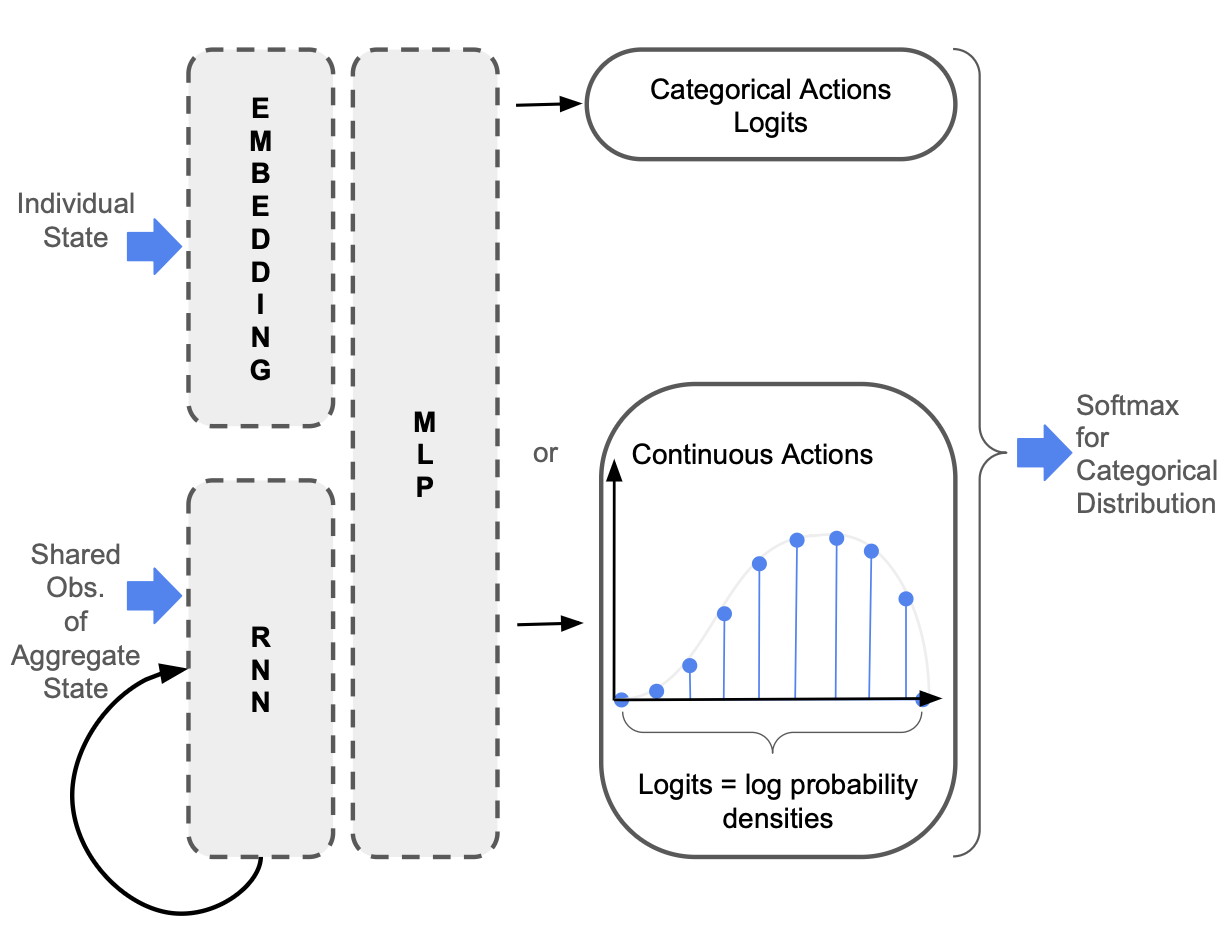
Figure 3: RSPG architecture: only the observations of the aggregate state are fed into the recurrent encoder such that the hidden state is independent of the individual state. This means that all agents share the same recurrent embedding at each timestep. In practice, we compute this embedding once per timestep and broadcast it to all states. For continuous actions, we parameterise an underlying continuous distribution to maintain ordinality in the action space.

In this way, RSPG is a history-aware HSM. This means that it both learns a history-dependent policy, leading to more realistic agent behaviour in partially observable settings, while also benefiting from low-variance updates.

MFAX: A JAX-Based Framework for MFGs

Finally, I'll briefly introduce MFAX, our open-source, JAX-based framework for MFGs designed to encourage more research into different MFG problem settings. Unlike existing libraries, MFAX:

Supports both analytic and sample-based mean-field updates, thereby allowing implementation of different MFG problem settings (e.g. low vs. high-dimensional individual state spaces).
Distinguishes between HSMs and RL-based methods: unlike RL-based methods, HSMs have white-box access to individual state transition dynamics.
Accelerates analytic mean-field updates by using a functional representation of matrix multiplication.
Supports more complex environments, such as with common noise, partial observability, and multiple initial mean-field distributions.

The Google Colab linked at the top of this post shows how analytic mean-field updates and RSPG are implemented in MFAX.